Math Graphics
In the basic course we saw the command for including a picture file. It was \includegraphics. Which is slightly odd, isn’t it? Why not just use the simpler picture or graphics?
Well, LaTeX does have a simple picture environment! But because the language was meant to typeset pieces with heavy use of math, this environment is reserved for mathematical graphics.
Within the picture environment, you can use a small list of commands to place different types of figures. When combined, they can generate complex mathematical graphics.
It’s similar to vector graphics, in case you understand that. It isn’t very difficult, it might just be a lot to take in at once. We’ll start off simple.
Starting the Picture Environment
It’s a regular environment, except for the fact that the arguments are delimited differently: with parentheses for brackets.
1\begin{picture}{width, height)(xOffset, yOffset)
2    % ... picture commands ...
3\end{picture}
These arguments are not regular LaTeX numbers with units! They refer to the amount of units within the picture. To length that holds this information is \unitlength, which you can change the way you’re used to.
1\setlength{\unitlength}{4pt}
2\begin{picture}(20,20)(0,0)
3    %Picture with width and height of 80pt
4    %But there's nothing in it, yes, let's change that!
5\end{picture}
The xOffset and yOffset set the coordinates of the lower left corner of the picture. In the example, the point (0,0) is used for the lower left corner, which means any negative coordinates would not be visible inside the picture.
This uses the mathematical way of viewing axes. Right = X positive, Up = Y positive.
If you’re used to other computer graphics, maybe programming or game development, you might be profoundly confused by this. In all those other situations, Down = Y positive. Try to clearly make this distinction in your head. LaTeX is for typesetting math.
Putting Graphics on the Page
To put graphics on the page, three very important commands are available.
Place object at position (x,y). (You’ll learn about all the math objects soon.)
1\put(x, y){object}Place n objects, starting at position (x,y), with deltaX and deltaY space between each object and the next.
1\multiput(x, y)(deltaX, deltaY){n}{object}Place a quadratic Bezier curve using the three data points you provide. Mostly used for drawing graphs. These curves are, sadly enough, beyond the scope of this tutorial.
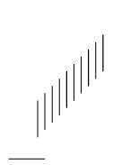
1\qbezier(x1, y1) (x2, y2) (x3, y3)1\setlength{\unitlength}{4pt}
2\begin{picture}(20,20)(0,0)
3 \put(0,0){\line(1,0){5}}
4 \multiput(4,3)(1,1){10}{\line(0,1){5}}
5\end{picture}
Changing Thickness
By default, lines have medium thickness. You can change this at any time. These commands take effect until a next one is encountered.
| Command | Description |
|---|---|
\thicklines | Slightly thicker lines |
\thinlines | Slightly thinner lines |
\linethickness{length} | Sets a custom line thickness |
Math Objects
As promised, here’s a list of all the math objects that can be placed within the picture:
| Command | Description |
|---|---|
\line(x, y){length} | Creates a line with length length, with direction vector (x,y). A direction vector can only take integers. |
\vector(x, y){length} | Also creates a line, but with an arrow at the end. |
\circle{diameter} | Creates a circle |
\circle*{diameter} | Creates a filled circle (a disk). |
\oval(width, height)[position] | Creates an oval. The optional argument position can be top, right, bottom or left (t, |
\frame{…} | Creates a rectangular frame around the object that’s inside, with no padding space. |
| Text or math | You can put any of the LaTeX you learned inside a picture—regular text and fancy math. This, however, only works for single lines. |
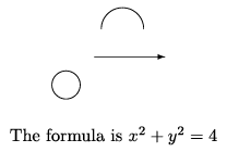
1\setlength{\unitlength}{4pt}
2\begin{picture}(20,20)(0,0)
3    \put(0,0){The formula is $x^2 + y^2 = 4$}
4    \put(8,8){\circle{4}}
5    \put(16,16){\oval(6,6)[t]}
6    \put(12,12){\vector(1,0){10}}
7\end{picture}
Save Boxes
If you want to reuse a certain (complex) graphic multiple times in your picture, you can save it in a save box.
Now you only need to define it once, and use it anywhere else by referencing the name under which you saved it. This is a very powerful way of creating pictures, which greatly reduces the time it takes to create them.
To declare a new save box, use
1\newsavebox{name}To define it, i.e. tell exactly what’s inside, use
1\savebox{name}(width, height)[position]{content}Put it in your picture wherever you want, and as many times as you like, using
1\usebox{name}1\setlength{\unitlength}{4pt}
2\begin{picture}(20,20)(0,0)
3 \newsavebox{MYBOX}
4 \savebox{MYBOX}(5,5)[l]{%
5 \put(0,0){\circle*{4}}
6 \put(1,0){\circle*{4}}
7 }
8 \put(10,10){\usebox{MYBOX}}
9\end{picture}
Want to support me?
Buy one of my projects. You get something nice, I get something nice.
Donate through a popular platform using the link below.
Simply giving feedback or spreading the word is also worth a lot.